x = np.linspace(0, 10, 100)
y = (x - 2.5) ** 2
fig, ax = plt.subplots(figsize=(3, 3))
ax.plot(x, y);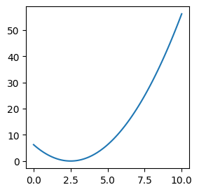
Adapted from:
The better calculus pedagogy is the calculus of infintesimals, that is: assume \(f'(x) = \frac{f(x + \Delta x)-f(x)}{\Delta x}\) like normal and ignore second order infinitesimals (i.e., infinitesimals of infinitesimals). By doing so, the main rules of arithmetic suddenly also apply to calculus. For example:
\[ \begin{align*} \frac{\Delta}{\Delta x} x^2 & = \frac{(x + \Delta x)^2 - x^2}{\Delta x} \\ & = \frac{x^2 + 2 x \Delta x + \Delta x^2 - x^2}{\Delta x} \\ & = \frac{2 x \Delta x + \Delta x^2}{\Delta x} \\ & = \frac{2 x \Delta x}{\Delta x} \\ & = 2x \end{align*} \]
(Fundamental theorem, distributivity, cancelling terms in numerator, second rule, cancelling shared term in numerator and denominator.)
\[ \begin{align*} \frac{\Delta y}{\Delta x} = \frac{\Delta y}{\Delta u} \left( \frac{\Delta u}{\Delta x} \right) \end{align*} \]
(Shared term in numerator and denominator.)
This is simple arithmetic! I’ve always found it a bit tricky to come up with a real-world, geometric example for this, as you need to come up with a function that depends on the output of another function. It’s a bit contrived, but this example is intuitive to me: imagine you’re on a walking side-walk, and someone pointing a speed radar at you and adjusting the speed of the sidewalk based on your speed. Mathematically, your speed is a product of your total velocity is the product of your walking velocity and the moving sidewalk velocity.
\[ \begin{align} \frac{\Delta C}{\Delta B} &= 2\\ \frac{\Delta B}{\Delta A} &= 4\\ \therefore \frac{\Delta C}{\Delta A} &= \frac{\Delta C}{\Delta B} \left( \frac{\Delta B}{\Delta A} \right) = 2 \times 4 = 8 \\ \end{align} \]
Here’s another intuitive demonstration of the chain rule, using chains (and gears): click here.
How does this relate to deep learning? Suppose we wanted to model this function with a neural network.
x = np.linspace(0, 10, 100)
y = (x - 2.5) ** 2
fig, ax = plt.subplots(figsize=(3, 3))
ax.plot(x, y);
A single line wouldn’t be especially adequate for this. (The sum of lines is just a line.) But what about the sum of rectified lines?
y1 = np.clip(-3 * (x - 2), a_min=0, a_max=None)
y2 = np.clip(3 * (x - 3), a_min=0, a_max=None)
y3 = np.clip(6 * (x - 5), a_min=0, a_max=None)

fig, (ax0, ax1) = plt.subplots(1, 2, figsize=(6, 3))
ax0.plot(x, y)
ax0.plot(x, y1)
ax0.plot(x, y2)
ax0.plot(x, y3)
ax1.plot(x, y)
ax1.plot(x, y1 + y2 + y3);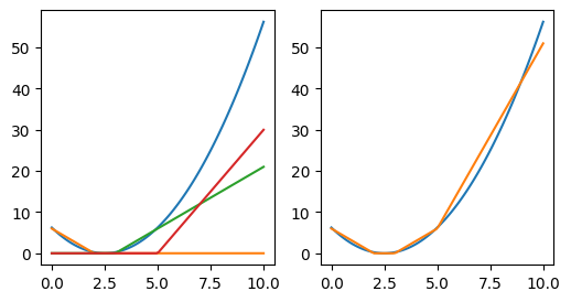
This is the idea of neural networks (except, instead of lines, we’re dealing with hyperplanes).
Let’s consider a specific problem. Suppose we wanted to classify digits with a simple neural network.
def MNISTDataModule(
    bs:int=128
):
MNIST data Module
It’s a bit cleaner to deal with images as vectors for this exercise.
X_trn = rearrange(X_trn, "b h w -> b (h w)")Say we wanted to classify a digit as a “seven” (or not) based on a single pixel. A trained linear model would find some coefficient and you would draw some line dividing sevens from non-sevens.
Of course, this is pretty limiting. What if this surface had a lot of curvature?
x = np.linspace(0, 1, 100)
y_t = 1 - x**2
y_pred = -0.95 * x + 1.1
fig, ax = plt.subplots(figsize=(3, 3))
ax.plot(x, y_t, label="True")
ax.plot(x, y_pred, label="Pred")
ax.set(xlabel="Pixel Intensity", ylabel="P(Seven)")
fig.legend();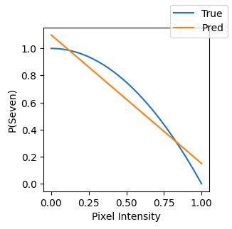
How do fit the sum of rectified lines like before?
To make this more interesting, let’s consider using all pixels, for all images.
Let’s define some parameters and helpers.
def relu(x):
    return np.clip(x, a_min=0, a_max=None)


n, m = X_trn.shape
nh = 50  # num. hidden dimensions
n, m
(60000, 784)Our results are going to be non-sense here, but this gives us the right dimensions for everything.
W0 = np.random.randn(m, nh)
b0 = np.zeros(nh)
W1 = np.random.randn(nh, 1)
b1 = np.zeros(1)

l0 = X_trn @ W0 + b0
l1 = relu(l0)
y_pred = l1 @ W1 + b1
y_pred[:5]
array([[ -9.87308795],
[-24.17324311],
[ 32.42885041],
[ 6.0755439 ],
[-65.67629667]])Let’s compute an regression loss to get the model to predict the label. (This isn’t formally apropriate but it gives us the intuition.)
y_pred.shape, y_true.shape((60000, 1), (60000,))diff = y_pred.T - y_true
mse = (diff**2).mean()
mse1979.1768273281134Eventually, at the end of the forward pass, we end up with a single number. We compute the loss for each example in the batch and take the batchwise mean or sum of the loss. Then, we use this along with the gradients with respect to each parameter to update the weights,
Let’s calculate these derivates, one by one 🤩
First, we need to determine the gradient of the loss with respect to it’s input.
\[MSE = \frac{ \sum_{i=1}^{N} ( y^i-a^i )^2 }{N}\]
This function composes an inner difference function and an outer square function. By the chain rule:
\[ \frac{d}{dx} f(g(x,y)) = f'(g(x,y)) g'(x,y) \]
Let \(g(x,y) = x-y\) and \(f(x) = \frac{x^2}{n}\)
Thus, \(\frac{d}{dx} g(x,y)=\frac{dx}{dx} - \frac{dy}{dx}=1\) and \[ \begin{align*} f'(g(x, y)) & = f'((x-y)^2 / n) \\ & = f'((x^2 - 2xy + y^2)/n) \\ & = (2x - 2y) / n \end{align*} \]
Let’s verify:
assert n == 60000
x, y = sympy.symbols("x y")
sympy.diff(((x - y) ** 2) / n, x)
\(\displaystyle \frac{x}{30000} - \frac{y}{30000}\)
Great. Now, to implement this in code, we need a way to store gradients on tensors themselves.
@dataclass
class T:
    """Wrapper for numpy arrays to help store a gradient"""

    value: Any
    g: Any = None

    def __getattr__(self, t):
        return getattr(self.value, t)

    def __getitem__(self, i):
        return self.value[i]

    @property
    def v(self):
        return self.value
Then, we can implement it like so:
def mse_grad(y_pred: T, y_true: np.array):
    diff = y_pred.squeeze() - y_true
    y_pred_g = 2 * diff / n
    y_pred.g = y_pred_g[:, None]
Continuing on with the linear transformation layer, we’ll review the mathematics then implement the code.
For a linear layer, the gradient is derived like so:
Let \(L = loss(Y)\) and \(Y = WX+B\) be a neural network. We want to compute the partial derivates of \(L\) with respect to \(W\), \(B\) and \(X\) to, ultimately, reduce \(L\).
Starting with a single, \(j\)th parameter of the \(i\)th example, \(x_j^i\)
\[ \begin{align*} \frac{\partial L}{\partial x_j^i} &= \frac{\partial L}{\partial Y} \cdot \frac{\partial Y}{\partial x_j^i} \\ &= \sum_{k=1}^{N} \frac{\partial L}{\partial y^k} \cdot \frac{\partial y^k}{\partial x_j^i} \end{align*} \]
Note that \(\frac{\partial y^k}{\partial x_j^i} = 0\) if \(k \neq i\) (i.e., the output of an example passed through the network is not a function of the input of a different example). Therefore,
\[ \begin{align*} \sum_{k=1}^{N} \frac{\partial L}{\partial y^k} \cdot \frac{\partial y^k}{\partial x_j^i} &= \frac{\partial L}{\partial y^i} \cdot \frac{\partial y^i}{\partial x_j^i} \\ &= \frac{\partial L}{\partial y^i} \cdot \frac{\partial w_j x_j^i +b}{\partial x_j^i} \\ &= \frac{\partial L}{\partial y^i} w_j \end{align*} \]
The matrix of derivates for all \(d\) parameters (\(j \in \{1, ..., d\}\)) and \(N\) examples (\(i \in \{1, ..., N\}\)) is:
\[ \frac{\partial L}{\partial X} = \begin{bmatrix} \frac{\partial L}{\partial y^1} w_1 & \dots & \frac{\partial L}{\partial y^1} w_d \\ \frac{\partial L}{\partial y^2} w_1 & \dots & \frac{\partial L}{\partial y^2} w_d \\ \vdots \\ \frac{\partial L}{\partial y^N} w_1 & \dots & \frac{\partial L}{\partial y^N} w_d \\ \end{bmatrix} = \begin{bmatrix} \frac{\partial L}{\partial y^1} \\ \frac{\partial L}{\partial y^2} \\ \vdots \\ \frac{\partial L}{\partial y^N} \\ \end{bmatrix} \begin{bmatrix} w_1 & w_2 & \dots & w_d \end{bmatrix} \]
In code: inp.g = out.g @ w.T
Starting with a single parameter, \(w_j\):
\[ \begin{align*} \frac{\partial L}{\partial w_j} &= \frac{\partial L}{\partial Y} \cdot \frac{\partial Y}{\partial w_j} \\ &= \sum_{k=1}^{N} \frac{\partial L}{\partial y^k} \cdot \frac{\partial y^k}{\partial w_j} \\ &= \sum_{k=1}^{N} \frac{\partial L}{\partial y^k} \cdot \frac{\partial w_j x_j^k + b_j}{\partial w_j} \\ &= \sum_{k=1}^{N} \frac{\partial L}{\partial y^k} x_j^k \end{align*} \]
For all parameters, \(W\):
\[ \frac{\partial L}{\partial W} = \begin{bmatrix} \frac{\partial L}{\partial w_{1}} \\ \frac{\partial L}{\partial w_{2}} \\ \vdots \\ \frac{\partial L}{\partial w_{d}} \end{bmatrix} = \begin{bmatrix} \sum_{k=1}^{N} \frac{\partial L}{\partial y^k} x_1^k \\ \sum_{k=1}^{N} \frac{\partial L}{\partial y^k} x_2^k \\ \vdots \\ \sum_{k=1}^{N} \frac{\partial L}{\partial y^k} x_d^k \end{bmatrix} = \begin{bmatrix} \frac{\partial L}{\partial y^1} x_1^1 &+ \dots &+ \frac{\partial L}{\partial y^N} x_1^N \\ \frac{\partial L}{\partial y^1} x_2^1 &+ \dots &+ \frac{\partial L}{\partial y^N} x_2^N \\ \vdots & \ddots & \vdots \\ \frac{\partial L}{\partial y^1} x_d^1 &+ \dots &+ \frac{\partial L}{\partial y^N} x_d^N \\ \end{bmatrix} = \begin{bmatrix} x_1^1 & \dots & x^{N}_1 \\ x_2^1 & \dots & x^{N}_2 \\ \vdots & \ddots & \vdots \\ x_d^1 & \dots & x^{N}_d \end{bmatrix} \begin{bmatrix} \frac{\partial L}{\partial y_{1}} \\ \frac{\partial L}{\partial y_{2}} \\ \vdots \\ \frac{\partial L}{\partial y_{N}} \\ \end{bmatrix} = X^T \frac{\partial L}{\partial Y} \]
In code: w.g = inp.v.T @ out.g
\[ \begin{align*} \frac{\partial L}{\partial B} &= \frac{\partial L}{\partial Y} \cdot \frac{\partial Y}{\partial B} \\ &= \sum_{k=1}^{N} \frac{\partial L}{\partial y^k} \cdot \frac{\partial y^k}{\partial B} \\ &= \sum_{k=1}^{N} \frac{\partial L}{\partial y^k} (1) \\ &= \sum_{k=1}^{N} \frac{\partial L}{\partial y^k} \end{align*} \]
In code b.g = out.g.sum(axis=0)
You can see that these derivation are similar to their single-variable counterparts (e.g. \(\frac{dL}{dm} = \frac{dL}{dy} \cdot \frac{dy}{dm} = \frac{dL}{dy} \cdot \frac{dmx+b}{dm}=\frac{dL}{dy}x\)). However, the order of operations and the transposition is dictated by the matrix mathematics.
In code:
def lin_grad(inp, out, w, b):
    inp.g = out.g @ w.T
    w.g = inp.v.T @ out.g
    b.g = out.g.sum(axis=0)
Much credit for my understanding goes to this blog bost and this article.
For ReLU, we pass the upstream gradient downstream for any dimensions that contributed to the upstream signal. Note that this is an element-wise operation because the layer operates only on specific elements and has no global behavior.
def relu_grad(inp, out):
    inp.g = (inp.value > 0).astype(float) * out.g
Putting it all together:
# "Tensorize" the weights, biases and outputs
tensors = (y_pred, W1, b1, l1, W0, b0, l0, X_trn)
ty_pred, tW1, tb1, tl1, tW0, tb0, tl0, tX_trn = map(T, tensors)
mse_grad(ty_pred, y_true)
ty_pred.g[:5]
array([[-0.00049577],
[-0.00080577],
[ 0.00094763],
[ 0.00016918],
[-0.00248921]])mse_grad(ty_pred, y_true)
lin_grad(tl1, ty_pred, tW1, tb1)
relu_grad(tl0, tl1)
lin_grad(tX_trn, tl0, tW0, tb0)Verify with PyTorch
# Port layers
pt_lin0 = nn.Linear(m, nh)
dtype = pt_lin0.weight.data.dtype
pt_lin0.weight.data = torch.from_numpy(tW0.v.T).to(dtype)
pt_lin0.bias.data = torch.from_numpy(tb0.v).to(dtype)
pt_lin1 = nn.Linear(nh, 1)
pt_lin1.weight.data = torch.from_numpy(tW1.T).to(dtype)
pt_lin1.bias.data = torch.from_numpy(tb1.v).to(dtype)

# Forward pass
logits = pt_lin0(torch.from_numpy(X_trn).to(dtype))
logits = F.relu(logits)
logits = pt_lin1(logits)
loss = F.mse_loss(
    logits.squeeze(),
    torch.from_numpy(y_true).float(),
)

# Backward pass
loss.backward()

for w, b, layer in [
    (tW0, tb0, pt_lin0),
    (tW1, tb1, pt_lin1),
]:
    assert torch.isclose(
        torch.from_numpy(w.g.T).float(),
        layer.weight.grad,
        atol=1e-4,
    ).all()
    assert torch.isclose(
        torch.from_numpy(b.g.T).float(),
        layer.bias.grad,
        atol=1e-4,
    ).all()
Let’s refactor these as classes.
class Module:
    def __call__(self, *x):
        self.inp = x
        self.out = self.forward(*x)
        if isinstance(self.out, (np.ndarray,)):
            self.out = T(self.out)
        return self.out


class ReLu(Module):
    def forward(self, x: T):
        return relu(x)

    def backward(self):
        (x,) = self.inp
        relu_grad(x, self.out)


class Linear(Module):
    def __init__(self, h_in, h_out):
        self.W = T(np.random.randn(h_in, h_out))
        self.b = T(np.zeros(h_out))

    def forward(self, x):
        return T(x @ self.W.v + self.b.v)

    def backward(self):
        (x,) = self.inp
        lin_grad(x, self.out, self.W, self.b)


class MSE(Module):
    def forward(self, y_pred, y_true):
        return ((y_pred.squeeze() - y_true) ** 2).mean()

    def backward(self):
        y_pred, y_true = self.inp
        mse_grad(y_pred, y_true)


class MLP(Module):
    def __init__(self, layers, criterion):
        super().__init__()
        self.layers = layers
        self.criterion = criterion

    def forward(self, x, y_pred):
        for l in self.layers:
            x = l(x)
        self.criterion(x, y_pred)

    def backward(self):
        self.criterion.backward()
        for l in reversed(self.layers):
            l.backward()


model = MLP([Linear(m, nh), ReLu(), Linear(nh, 1)], criterion=MSE())
model(tX_trn, y_true)
model.backward()This is quite a bit cleaner!
By the rules of FastAI, we can now use the torch.nn.Module classes which is the equivalent in PyTorch.