Tiny Imagenet (Part I)

Scaling up the dataset and training a UNet model

Adapted from

• https://www.youtube.com/watch?v=z1In7QaG0fg

---

source

tiny_imagenet

 tiny_imagenet (dir_=Path('../tiny-imagenet-200'))

# Download, if needed
tiny_imagenet();

---

source

TinyImageNetDatasetGenerator

 TinyImageNetDatasetGenerator (base_dir=None)

Generate Tiny Imagenet rows lazily from zip file

upload = False
if upload:
    dg = TinyImageNetDatasetGenerator()
    splits = {}
    for split, split_gen in [("train", dg.gen_train), ("test", dg.gen_test)]:
        # Ensure at least one record
        next(iter(split_gen()))
        ds = Dataset.from_generator(split_gen)
        ds = ds.cast_column("image", DatasetsImage())
        splits[split] = ds
    dsd = DatasetDict(splits)
    dsd.push_to_hub("jeremyf/tiny-imagent-200")

---

source

tiny_imagenet_dataset_dict

 tiny_imagenet_dataset_dict ()

Huggingface dataset from the HF hub

---

source

to_rgb

 to_rgb (img)

---

source

norm

 norm (x)

---

source

denorm

 denorm (x)

---

source

preprocess_factory

 preprocess_factory (pipe_)

---

source

get_imagenet_dls

 get_imagenet_dls (bs=512, with_word=False,
                   training_preprocessor=[<function to_rgb at
                   0x7f2095257640>, PILToTensor(), ConvertImageDtype(),
                   <function norm at 0x7f2095257760>])

dls = get_imagenet_dls(with_word=True)

Downloading readme: 100%|██████████████████████| 453/453 [00:00<00:00, 1.30MB/s]
Downloading data files:   0%|                             | 0/2 [00:00<?, ?it/s]
Downloading data:   0%|                              | 0.00/158M [00:00<?, ?B/s]
Downloading data:   3%|▌                    | 4.19M/158M [00:03<01:57, 1.31MB/s]
Downloading data:   8%|█▋                   | 12.6M/158M [00:06<01:06, 2.19MB/s]
Downloading data:  13%|██▊                  | 21.0M/158M [00:09<00:56, 2.43MB/s]
Downloading data:  19%|███▉                 | 29.4M/158M [00:13<00:55, 2.32MB/s]
Downloading data:  24%|█████                | 37.7M/158M [00:16<00:50, 2.39MB/s]
Downloading data:  29%|██████▏              | 46.1M/158M [00:19<00:45, 2.43MB/s]
Downloading data:  35%|███████▎             | 54.5M/158M [00:21<00:37, 2.77MB/s]
Downloading data:  40%|████████▍            | 62.9M/158M [00:24<00:30, 3.07MB/s]
Downloading data:  45%|█████████▌           | 71.3M/158M [00:27<00:30, 2.82MB/s]
Downloading data:  51%|██████████▋          | 79.7M/158M [00:31<00:30, 2.57MB/s]
Downloading data:  56%|███████████▋         | 88.1M/158M [00:34<00:25, 2.72MB/s]
Downloading data:  61%|████████████▊        | 96.5M/158M [00:36<00:21, 2.83MB/s]
Downloading data:  67%|██████████████▋       | 105M/158M [00:39<00:17, 3.04MB/s]
Downloading data:  72%|███████████████▊      | 113M/158M [00:42<00:14, 2.97MB/s]
Downloading data:  77%|████████████████▉     | 122M/158M [00:45<00:12, 2.90MB/s]
Downloading data:  83%|██████████████████▏   | 130M/158M [00:47<00:09, 2.93MB/s]
Downloading data:  88%|███████████████████▎  | 138M/158M [00:51<00:06, 2.83MB/s]
Downloading data:  93%|████████████████████▌ | 147M/158M [00:56<00:04, 2.18MB/s]
Downloading data: 100%|██████████████████████| 158M/158M [00:59<00:00, 2.65MB/s]
Downloading data files:  50%|██████████▌          | 1/2 [00:59<00:59, 59.44s/it]
Downloading data:   0%|                             | 0.00/15.8M [00:00<?, ?B/s]
Downloading data:  26%|█████▎              | 4.19M/15.8M [00:02<00:07, 1.46MB/s]
Downloading data: 100%|████████████████████| 15.8M/15.8M [00:05<00:00, 2.97MB/s]
Downloading data files: 100%|█████████████████████| 2/2 [01:04<00:00, 32.39s/it]
Extracting data files: 100%|█████████████████████| 2/2 [00:00<00:00, 614.82it/s]
Generating train split: 100%|█| 100000/100000 [00:00<00:00, 233408.11 examples/s
Generating test split: 100%|███| 10000/10000 [00:00<00:00, 665783.68 examples/s]
Map: 100%|████████████████████████| 10000/10000 [00:10<00:00, 913.89 examples/s]

CPU times: user 12.4 s, sys: 2.92 s, total: 15.3 s
Wall time: 1min 20s

---

source

viz

 viz (dls)

viz(dls)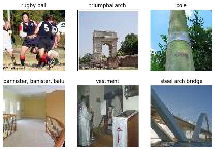

xb, _, words = dls.peek()
pixels = xb.reshape(-1)
pixels = pixels[torch.randperm(len(pixels))]
plt.hist(pixels[:1000], bins=25);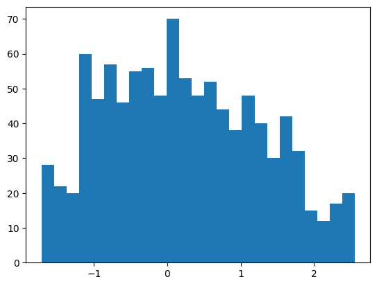

xb.min(), xb.max()

(tensor(-1.7143), tensor(2.5556))

Let’s implement the model with color and a slightly fancier final pooling layer.

nn.AdaptiveAvgPool2d?

Init signature:
nn.AdaptiveAvgPool2d(
    output_size: Union[int, NoneType, Tuple[Optional[int], ...]],
) -> None
Docstring:     
Applies a 2D adaptive average pooling over an input signal composed of several input planes.
The output is of size H x W, for any input size.
The number of output features is equal to the number of input planes.
Args:
    output_size: the target output size of the image of the form H x W.
                 Can be a tuple (H, W) or a single H for a square image H x H.
                 H and W can be either a ``int``, or ``None`` which means the size will
                 be the same as that of the input.
Shape:
    - Input: :math:`(N, C, H_{in}, W_{in})` or :math:`(C, H_{in}, W_{in})`.
    - Output: :math:`(N, C, S_{0}, S_{1})` or :math:`(C, S_{0}, S_{1})`, where
      :math:`S=\text{output\_size}`.
Examples:
    >>> # target output size of 5x7
    >>> m = nn.AdaptiveAvgPool2d((5, 7))
    >>> input = torch.randn(1, 64, 8, 9)
    >>> output = m(input)
    >>> # target output size of 7x7 (square)
    >>> m = nn.AdaptiveAvgPool2d(7)
    >>> input = torch.randn(1, 64, 10, 9)
    >>> output = m(input)
    >>> # target output size of 10x7
    >>> m = nn.AdaptiveAvgPool2d((None, 7))
    >>> input = torch.randn(1, 64, 10, 9)
    >>> output = m(input)
Init docstring: Initializes internal Module state, shared by both nn.Module and ScriptModule.
File:           ~/micromamba/envs/slowai/lib/python3.11/site-packages/torch/nn/modules/pooling.py
Type:           type
Subclasses:     

class TinyImageResNet1(nn.Module):
    def __init__(
        self,
        nfs,
        n_outputs=10,
        p_drop=0.1,
    ):
        super().__init__()
        self.nfs = nfs
        self.n_outputs = n_outputs
        self.layers = nn.Sequential(*self.get_layers(nfs, n_outputs))
        self.pool = nn.Sequential(
            nn.AdaptiveAvgPool2d(output_size=1),
            nn.Flatten(),
        )
        self.drop = nn.Dropout(p_drop)
        self.lin = nn.Linear(nfs[-1], n_outputs, bias=False)
        self.norm = nn.BatchNorm1d(n_outputs)

    def get_layers(self, nfs, n_outputs=10):
        layers = [Conv(3, nfs[0], ks=5, stride=1)]
        for c_in, c_out in zip(nfs, nfs[1:]):
            block = ResidualConvBlock(c_in, c_out)
            layers.append(block)
        return layers

    def forward(self, x):
        x = self.layers(x)
        x = self.pool(x)
        x = self.drop(x)
        x = self.lin(x)
        x = self.norm(x)
        return x

    @classmethod
    def kaiming(cls, *args, **kwargs):
        model = cls(*args, **kwargs)
        model.apply(init_leaky_weights)
        return model

dls = get_imagenet_dls(bs=512)  # We don't want the human-readable labels

model = TinyImageResNet1.kaiming(
    n_outputs=200,
    nfs=[32, 64, 128, 256, 512, 1024],
)
summarize(model, [*model.layers, model.lin, model.norm], get_imagenet_dls())

Type	Input	Output	N. params	MFlops
Conv	(512, 3, 64, 64)	(512, 32, 64, 64)	2,464	9.8
ResidualConvBlock	(512, 32, 64, 64)	(512, 64, 32, 32)	57,664	58.7
ResidualConvBlock	(512, 64, 32, 32)	(512, 128, 16, 16)	230,016	58.7
ResidualConvBlock	(512, 128, 16, 16)	(512, 256, 8, 8)	918,784	58.7
ResidualConvBlock	(512, 256, 8, 8)	(512, 512, 4, 4)	3,672,576	58.7
ResidualConvBlock	(512, 512, 4, 4)	(512, 1024, 2, 2)	14,685,184	58.7
Linear	(512, 1024)	(512, 200)	204,800	0.2
BatchNorm1d	(512, 200)	(512, 200)	400	0.0
Total			19,771,888	303.646864

---

source

lr_find

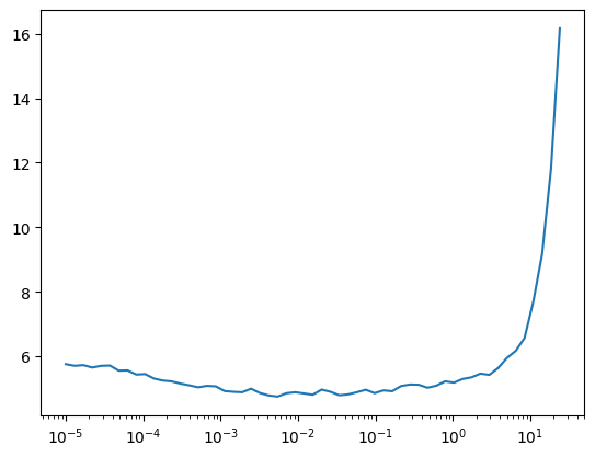
 lr_find (model, dls, start_lr, gamma=1.3, n_epochs=2, extra_cbs=(),
          loss_fn=<function cross_entropy>)

lr_find(model, dls, start_lr=1e-5)

0.00% [0/2 00:00<?]

28.57% [56/196 00:08<00:21 11.806]

---

source

train

 train (model, dls, lr=0.01, n_epochs=2, extra_cbs=())

model = TinyImageResNet1.kaiming(
    n_outputs=200,
    nfs=[32, 64, 128, 256, 512, 1024],
)
train(model, dls, lr=0.1, n_epochs=25)

MulticlassAccuracy	loss	epoch	train
0.081	4.524	0	train
0.119	4.143	0	eval
0.180	3.747	1	train
0.182	3.735	1	eval
0.242	3.359	2	train
0.193	3.809	2	eval
0.284	3.119	3	train
0.189	3.818	3	eval
0.312	2.964	4	train
0.178	4.275	4	eval
0.334	2.843	5	train
0.159	4.461	5	eval
0.357	2.724	6	train
0.137	4.707	6	eval
0.374	2.626	7	train
0.179	4.110	7	eval
0.397	2.514	8	train
0.124	4.837	8	eval
0.417	2.420	9	train
0.199	4.202	9	eval
0.437	2.314	10	train
0.191	3.961	10	eval
0.458	2.207	11	train
0.215	3.956	11	eval
0.478	2.110	12	train
0.237	3.711	12	eval
0.505	1.986	13	train
0.251	3.702	13	eval
0.537	1.833	14	train
0.241	4.379	14	eval
0.569	1.680	15	train
0.172	6.307	15	eval
0.607	1.497	16	train
0.208	4.592	16	eval
0.664	1.261	17	train
0.310	3.490	17	eval
0.733	0.972	18	train
0.312	3.723	18	eval
0.819	0.654	19	train
0.338	3.578	19	eval
0.914	0.325	20	train
0.398	3.102	20	eval
0.976	0.113	21	train
0.437	2.950	21	eval
0.997	0.033	22	train
0.441	2.972	22	eval
0.999	0.015	23	train
0.440	2.966	23	eval
1.000	0.012	24	train
0.441	2.969	24	eval

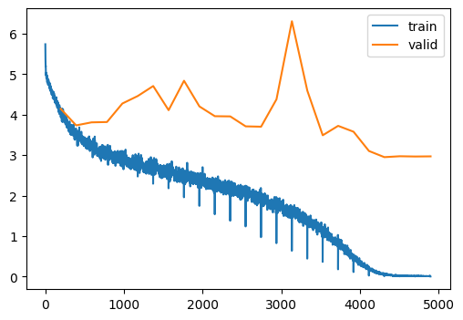
That’s clearly overfitting. Let’s add some minor augmentation.

T.RandomErasing?

Init signature:
T.RandomErasing(
    p=0.5,
    scale=(0.02, 0.33),
    ratio=(0.3, 3.3),
    value=0,
    inplace=False,
)
Docstring:     
Randomly selects a rectangle region in a torch.Tensor image and erases its pixels.
This transform does not support PIL Image.
'Random Erasing Data Augmentation' by Zhong et al. See https://arxiv.org/abs/1708.04896
Args:
     p: probability that the random erasing operation will be performed.
     scale: range of proportion of erased area against input image.
     ratio: range of aspect ratio of erased area.
     value: erasing value. Default is 0. If a single int, it is used to
        erase all pixels. If a tuple of length 3, it is used to erase
        R, G, B channels respectively.
        If a str of 'random', erasing each pixel with random values.
     inplace: boolean to make this transform inplace. Default set to False.
Returns:
    Erased Image.
Example:
    >>> transform = transforms.Compose([
    >>>   transforms.RandomHorizontalFlip(),
    >>>   transforms.PILToTensor(),
    >>>   transforms.ConvertImageDtype(torch.float),
    >>>   transforms.Normalize((0.485, 0.456, 0.406), (0.229, 0.224, 0.225)),
    >>>   transforms.RandomErasing(),
    >>> ])
Init docstring: Initializes internal Module state, shared by both nn.Module and ScriptModule.
File:           ~/micromamba/envs/slowai/lib/python3.11/site-packages/torchvision/transforms/transforms.py
Type:           type
Subclasses:     

dls = get_imagenet_dls(bs=512, training_preprocessor=preprocess_and_augment)
viz(dls)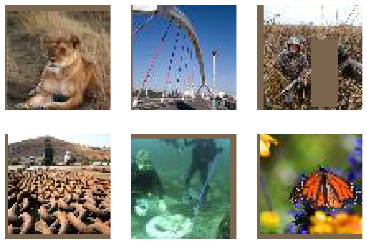

model = TinyImageResNet1.kaiming(
    n_outputs=200,
    nfs=[32, 64, 128, 256, 512, 1024],
)
train(model, dls, lr=0.1, n_epochs=25)

MulticlassAccuracy	loss	epoch	train
0.078	4.541	0	train
0.129	4.056	0	eval
0.166	3.847	1	train
0.154	4.086	1	eval
0.210	3.532	2	train
0.179	3.950	2	eval
0.247	3.317	3	train
0.174	3.973	3	eval
0.271	3.178	4	train
0.186	3.907	4	eval
0.297	3.037	5	train
0.227	3.507	5	eval
0.313	2.945	6	train
0.221	3.579	6	eval
0.330	2.852	7	train
0.190	3.795	7	eval
0.351	2.744	8	train
0.214	3.588	8	eval
0.367	2.667	9	train
0.185	3.882	9	eval
0.383	2.590	10	train
0.232	3.654	10	eval
0.399	2.511	11	train
0.218	3.653	11	eval
0.416	2.423	12	train
0.286	3.208	12	eval
0.434	2.345	13	train
0.295	3.322	13	eval
0.453	2.251	14	train
0.368	2.786	14	eval
0.471	2.153	15	train
0.301	3.272	15	eval
0.498	2.039	16	train
0.360	2.885	16	eval
0.522	1.912	17	train
0.431	2.474	17	eval
0.556	1.765	18	train
0.403	2.818	18	eval
0.588	1.615	19	train
0.456	2.405	19	eval
0.628	1.436	20	train
0.503	2.159	20	eval
0.672	1.253	21	train
0.537	2.000	21	eval
0.713	1.091	22	train
0.575	1.820	22	eval
0.745	0.961	23	train
0.592	1.762	23	eval
0.768	0.881	24	train
0.593	1.752	24	eval

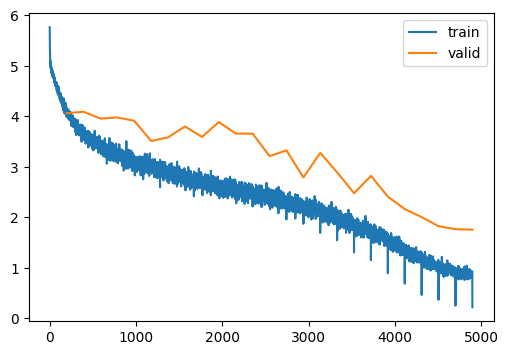
It does seem that augmentation is critical for performance. Compare 58.6% accuracy (mine) vs 59.3% accuracy (Howard).

How much better can we do?

Going deeper

To answer this, we can check Papers With Code. The best approach documented there is the ResNext paper at 72% accurate. This benchmark has shifted since the original course publication date, but here is the paper Jeremy refers to.

So, how much work is involved in going from 60% accurate to 70% accurate? “Real resnets” have multiple ResBlocks at the same feature map resolution.

n_blocks = (3, 2, 2, 1, 1)

This specification has five downsampling layers but nine ResBlocks

---

source

StackableResidualConvBlock

 StackableResidualConvBlock (n_blocks, c_in, c_out, conv_cls=<class
                             'slowai.resnets.ResidualConvBlock'>)

*A sequential container.

Modules will be added to it in the order they are passed in the constructor. Alternatively, an OrderedDict of modules can be passed in. The forward() method of Sequential accepts any input and forwards it to the first module it contains. It then “chains” outputs to inputs sequentially for each subsequent module, finally returning the output of the last module.

The value a Sequential provides over manually calling a sequence of modules is that it allows treating the whole container as a single module, such that performing a transformation on the Sequential applies to each of the modules it stores (which are each a registered submodule of the Sequential).

What’s the difference between a Sequential and a :class:torch.nn.ModuleList? A ModuleList is exactly what it sounds like–a list for storing Module s! On the other hand, the layers in a Sequential are connected in a cascading way.

Example::

# Using Sequential to create a small model. When `model` is run,
# input will first be passed to `Conv2d(1,20,5)`. The output of
# `Conv2d(1,20,5)` will be used as the input to the first
# `ReLU`; the output of the first `ReLU` will become the input
# for `Conv2d(20,64,5)`. Finally, the output of
# `Conv2d(20,64,5)` will be used as input to the second `ReLU`
model = nn.Sequential(
          nn.Conv2d(1,20,5),
          nn.ReLU(),
          nn.Conv2d(20,64,5),
          nn.ReLU()
        )

# Using Sequential with OrderedDict. This is functionally the
# same as the above code
model = nn.Sequential(OrderedDict([
          ('conv1', nn.Conv2d(1,20,5)),
          ('relu1', nn.ReLU()),
          ('conv2', nn.Conv2d(20,64,5)),
          ('relu2', nn.ReLU())
        ]))*

This was a tricky module to implement. Make sure that the channel, height and width dimensions are apropriate for all values of n_blocks.

class TinyImageResNet2(TinyImageResNet1):
    def __init__(
        self,
        nfs,
        n_blocks,
        n_outputs=10,
        p_drop=0.1,
    ):
        self.n_blocks = n_blocks
        super().__init__(nfs, n_outputs, p_drop)

    def get_layers(self, nfs, n_outputs=10):
        layers = [Conv(3, nfs[0], stride=1, ks=5)]
        for c_in, c_out, n_blocks in zip(nfs, nfs[1:], self.n_blocks):
            layers.append(StackableResidualConvBlock(n_blocks, c_in, c_out))
        return layers

model = TinyImageResNet2.kaiming(
    n_outputs=200,
    nfs=[32, 64, 128, 256, 512, 1024],
    n_blocks=n_blocks,
)
summarize(model, [*model.layers, model.lin, model.norm], dls)

Type	Input	Output	N. params	MFlops
Conv	(512, 3, 64, 64)	(512, 32, 64, 64)	2,464	9.8
StackableResidualConvBlock	(512, 32, 64, 64)	(512, 64, 32, 32)	213,952	218.1
StackableResidualConvBlock	(512, 64, 32, 32)	(512, 128, 16, 16)	541,952	138.4
StackableResidualConvBlock	(512, 128, 16, 16)	(512, 256, 8, 8)	2,165,248	138.4
StackableResidualConvBlock	(512, 256, 8, 8)	(512, 512, 4, 4)	3,672,576	58.7
StackableResidualConvBlock	(512, 512, 4, 4)	(512, 1024, 2, 2)	14,685,184	58.7
Linear	(512, 1024)	(512, 200)	204,800	0.2
BatchNorm1d	(512, 200)	(512, 200)	400	0.0
Total			21,486,576	622.416528

train(model, dls, lr=0.1, n_epochs=25)

MulticlassAccuracy	loss	epoch	train
0.068	4.621	0	train
0.101	4.285	0	eval
0.160	3.876	1	train
0.187	3.676	1	eval
0.226	3.429	2	train
0.221	3.561	2	eval
0.277	3.138	3	train
0.222	3.567	3	eval
0.312	2.952	4	train
0.283	3.124	4	eval
0.339	2.806	5	train
0.269	3.274	5	eval
0.360	2.696	6	train
0.225	3.778	6	eval
0.383	2.586	7	train
0.290	3.208	7	eval
0.400	2.494	8	train
0.293	3.169	8	eval
0.419	2.405	9	train
0.324	3.169	9	eval
0.437	2.322	10	train
0.356	2.849	10	eval
0.454	2.236	11	train
0.291	3.322	11	eval
0.471	2.162	12	train
0.352	2.957	12	eval
0.490	2.068	13	train
0.326	3.154	13	eval
0.510	1.976	14	train
0.352	2.911	14	eval
0.534	1.864	15	train
0.390	2.655	15	eval
0.560	1.743	16	train
0.442	2.527	16	eval
0.589	1.611	17	train
0.455	2.454	17	eval
0.620	1.470	18	train
0.498	2.181	18	eval
0.658	1.306	19	train
0.514	2.130	19	eval
0.704	1.113	20	train
0.529	2.054	20	eval
0.751	0.924	21	train
0.583	1.807	21	eval
0.803	0.734	22	train
0.599	1.746	22	eval
0.838	0.607	23	train
0.613	1.712	23	eval
0.860	0.533	24	train
0.614	1.706	24	eval

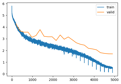
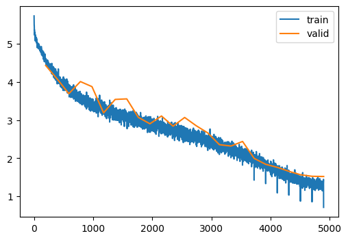
Yet more augmentation

T.TrivialAugmentWide?

Init signature:
T.TrivialAugmentWide(
    num_magnitude_bins: int = 31,
    interpolation: torchvision.transforms.functional.InterpolationMode = <InterpolationMode.NEAREST: 'nearest'>,
    fill: Optional[List[float]] = None,
) -> None
Docstring:     
Dataset-independent data-augmentation with TrivialAugment Wide, as described in
`"TrivialAugment: Tuning-free Yet State-of-the-Art Data Augmentation" <https://arxiv.org/abs/2103.10158>`_.
If the image is torch Tensor, it should be of type torch.uint8, and it is expected
to have [..., 1 or 3, H, W] shape, where ... means an arbitrary number of leading dimensions.
If img is PIL Image, it is expected to be in mode "L" or "RGB".
Args:
    num_magnitude_bins (int): The number of different magnitude values.
    interpolation (InterpolationMode): Desired interpolation enum defined by
        :class:`torchvision.transforms.InterpolationMode`. Default is ``InterpolationMode.NEAREST``.
        If input is Tensor, only ``InterpolationMode.NEAREST``, ``InterpolationMode.BILINEAR`` are supported.
    fill (sequence or number, optional): Pixel fill value for the area outside the transformed
        image. If given a number, the value is used for all bands respectively.
Init docstring: Initializes internal Module state, shared by both nn.Module and ScriptModule.
File:           ~/micromamba/envs/slowai/lib/python3.11/site-packages/torchvision/transforms/autoaugment.py
Type:           type
Subclasses:     

dls = get_imagenet_dls(bs=512, training_preprocessor=preprocess_and_trivial_augment)
viz(dls)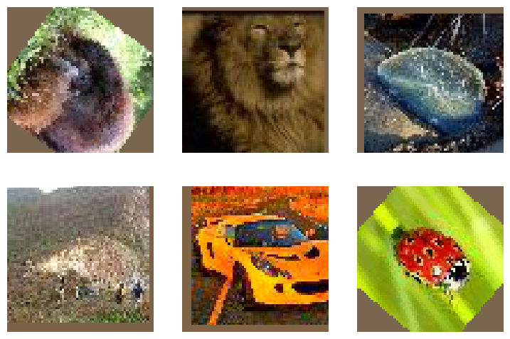

model = TinyImageResNet2.kaiming(
    n_outputs=200,
    nfs=[32, 64, 128, 256, 512, 1024],
    n_blocks=n_blocks,
)
summarize(model, [*model.layers, model.lin, model.norm], dls)

Type	Input	Output	N. params	MFlops
Conv	(512, 3, 64, 64)	(512, 32, 64, 64)	2,464	9.8
StackableResidualConvBlock	(512, 32, 64, 64)	(512, 64, 32, 32)	213,952	218.1
StackableResidualConvBlock	(512, 64, 32, 32)	(512, 128, 16, 16)	541,952	138.4
StackableResidualConvBlock	(512, 128, 16, 16)	(512, 256, 8, 8)	2,165,248	138.4
StackableResidualConvBlock	(512, 256, 8, 8)	(512, 512, 4, 4)	3,672,576	58.7
StackableResidualConvBlock	(512, 512, 4, 4)	(512, 1024, 2, 2)	14,685,184	58.7
Linear	(512, 1024)	(512, 200)	204,800	0.2
BatchNorm1d	(512, 200)	(512, 200)	400	0.0
Total			21,486,576	622.416528

train(model, dls, lr=0.1, n_epochs=25)

MulticlassAccuracy	loss	epoch	train
0.040	4.902	0	train
0.075	4.431	0	eval
0.097	4.338	1	train
0.136	4.074	1	eval
0.147	3.954	2	train
0.180	3.691	2	eval
0.189	3.684	3	train
0.161	4.008	3	eval
0.223	3.488	4	train
0.193	3.875	4	eval
0.244	3.360	5	train
0.270	3.188	5	eval
0.266	3.237	6	train
0.256	3.541	6	eval
0.285	3.128	7	train
0.242	3.555	7	eval
0.305	3.023	8	train
0.302	3.071	8	eval
0.323	2.937	9	train
0.322	2.903	9	eval
0.338	2.860	10	train
0.300	3.106	10	eval
0.355	2.770	11	train
0.340	2.840	11	eval
0.369	2.690	12	train
0.320	3.068	12	eval
0.388	2.598	13	train
0.358	2.851	13	eval
0.404	2.512	14	train
0.377	2.662	14	eval
0.428	2.402	15	train
0.442	2.354	15	eval
0.450	2.293	16	train
0.451	2.319	16	eval
0.473	2.178	17	train
0.433	2.439	17	eval
0.501	2.047	18	train
0.521	1.995	18	eval
0.532	1.894	19	train
0.555	1.840	19	eval
0.566	1.747	20	train
0.570	1.761	20	eval
0.600	1.602	21	train
0.598	1.657	21	eval
0.630	1.464	22	train
0.617	1.567	22	eval
0.656	1.358	23	train
0.627	1.526	23	eval
0.669	1.307	24	train
0.629	1.521	24	eval

torch.save(model, "../models/tiny_imagenet_200_classifier.pt")

Continued in part 2…