Initializations

Weights should be initialized apropriately

Adapted from:

• https://www.youtube.com/watch?v=vGsc_NbU7xc&t=129s

set_seed(42)
plt.style.use("ggplot")

Probability, misc

Topic	Description	Formula
Average Error	Typically 0 because positive and negative errors cancel out, making this metric not useful.	$ = y_{true} - y_{pred} $
Variance	The expected value of the squared deviation from the mean of a random variable.	\(\sigma^2 = \sum \frac{(x-\mathbb{E}[X])^2}{N}\) \(\sigma^2 = \mathbb{E}[X^2] - \mathbb{E}[X]^2\)
Covariance	A measure of the joint variability of two random variables.	\(\operatorname{cov}(X,Y) = \operatorname{E}{\big[(X - \operatorname{E}[X])(Y - \operatorname{E}[Y])\big]}\)
Pearson Correlation Coefficient	A normalized measure of the linear relationship between two variables.	\(\rho_{X,Y}= \frac{\operatorname{cov}(X,Y)}{\sigma_X \sigma_Y}\)

Baseline

Let’s look at a fashion MNIST classification problem. Our goal is to get accuracy to at least 90%.

class CNN(nn.Module):
    """Six layer convolutional neural network"""

    def __init__(self):
        super().__init__()
        self.layers = nn.Sequential(
            Conv2dWithReLU(1, 8, kernel_size=5, stride=2, padding=2),  # 14x14
            Conv2dWithReLU(8, 16, kernel_size=3, stride=2, padding=1),  # 7x7
            Conv2dWithReLU(16, 32, kernel_size=3, stride=2, padding=1),  # 4x4
            Conv2dWithReLU(32, 64, kernel_size=3, stride=2, padding=1),  # 2x2
            nn.Conv2d(64, 10, kernel_size=3, stride=2, padding=1),  # 1x1
        )

    def forward(self, x):
        x = self.layers(x)
        return rearrange(x, "bs c w h -> bs (c w h)")

Let’s start by finding the learning rate.

This diverges very quickly

TrainLearner(
    CNN(),
    fashion_mnist(),
    F.cross_entropy,
    lr=0.6,
    cbs=[LRFinderCB(), MomentumCB()],
).fit()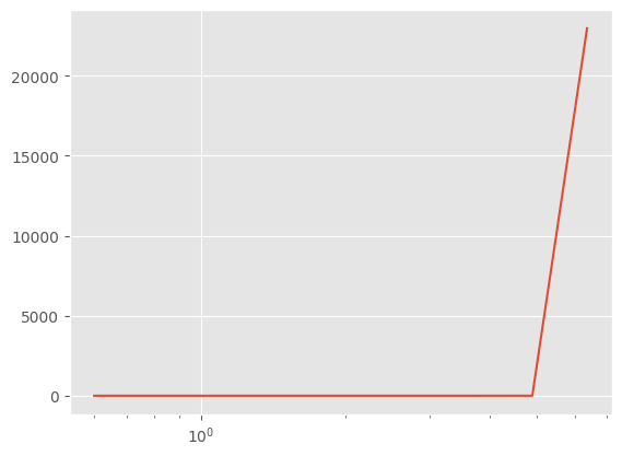

That’s unusable. Let’s dial down the learning rate increase and start at a lower learning rate.

LRFinderCB?

Init signature: LRFinderCB(gamma=1.3, max_mult=3)
Docstring:     
Find an apopriate learning rate by increasing it by a constant factor for each batch
until the loss diverges
File:           ~/Desktop/SlowAI/nbs/slowai/learner.py
Type:           type
Subclasses:     

TrainLearner(
    CNN(),
    fashion_mnist(64),
    F.cross_entropy,
    lr=1e-2,
    cbs=[LRFinderCB(gamma=1.05), MomentumCB()],
).fit()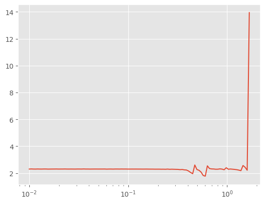

model = CNN()
stats = StoreModuleStatsCB(mods=model.layers)
cbs = [
    MomentumCB(),
    MetricsCB(MulticlassAccuracy(num_classes=10)),
    DeviceCB(),
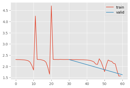
    ProgressCB(plot=True),
    stats,
]
TrainLearner(
    model,
    fashion_mnist(),
    F.cross_entropy,
    lr=0.6,
    cbs=cbs,
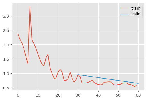
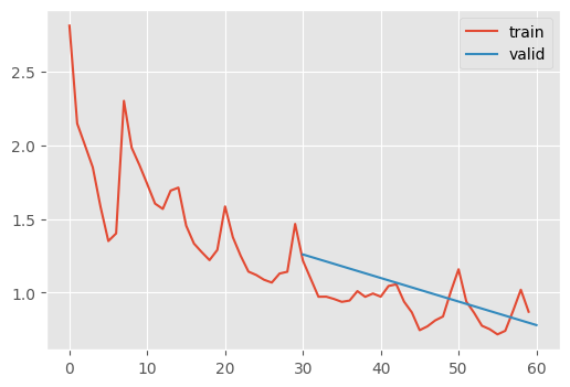
).fit(2)

MulticlassAccuracy	loss	epoch	train
0.168	2.378	0	train
0.100	2.301	0	eval
0.203	2.170	1	train
0.489	1.624	1	eval

stats.hist_plot()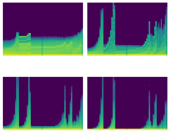

The issue with neural networks in real life is that they must be represented by discrete data structures. These can overflow…

x = torch.randn(200, 100)
for i in range(50):
    x = x @ torch.randn(100, 100)
x[0:5, 0:5]

tensor([[nan, nan, nan, nan, nan],
        [nan, nan, nan, nan, nan],
        [nan, nan, nan, nan, nan],
        [nan, nan, nan, nan, nan],
        [nan, nan, nan, nan, nan]])

…or underflow..

x = torch.randn(200, 100)
for i in range(50):
    x = x @ torch.randn(100, 100) * 0.01
x[0:5, 0:5]

tensor([[0., 0., 0., 0., 0.],
        [0., 0., 0., 0., 0.],
        [0., 0., 0., 0., 0.],
        [0., 0., 0., 0., 0.],
        [0., 0., 0., 0., 0.]])

We should scale our weights such that, throughout the training process, the mean remains near 0 and the standard deviation remains near 1. Otherwise, we are suseptible to these “dead units”

Glorot/Xavier

Normally, the mean variance of a layer is approximately the number of output dimensions

for d in [1, 100]:
    means = []
    sqrs = []

    for _ in range(500):
        x = torch.randn(d)
        a = torch.randn(512, d)
        y = a @ x
        means.append(y.mean())
        sqrs.append(y.pow(2).mean())

    res = torch.stack(means).mean(), torch.stack(sqrs).mean()
    print(res)

(tensor(-0.0011), tensor(1.1372))
(tensor(-0.0029), tensor(100.2205))

To encourage of variance of 1, the paper from Xavier Glorot and Yoshua Bengio proposed that each layer have a coefficient of \(\frac{1}{\sqrt{d}}\) where \(d\) is the number of inputs

d = 100
x = torch.randn(200, d)
for i in range(50):
    layer = torch.randn(d, d) * (1 / math.sqrt(d))
    x = x @ layer
x[0:5, 0:5]

tensor([[ 1.7367, -0.3418, -2.1874, -0.9467,  1.0451],
        [ 0.7802,  0.3702, -0.9278,  0.1607,  0.7578],
        [-2.0552,  1.0210,  1.7889,  0.1260, -1.0092],
        [-0.4922, -0.1349,  0.0443, -0.3037, -0.1711],
        [ 0.0103,  0.0468, -0.6201, -1.1773,  0.1258]])

Indeed, this gives us reasonable numbers! However, this doesn’t work for modern deep learning because of the activation layers.

Kaiming/He init

Notice that the first layer of a neural network has a favorable activation distribution

d1, d2 = 100, 100
x = torch.randn(200, d1)
y = torch.randn(200)
w = torch.randn(d1, d2) / math.sqrt(d1)
b = torch.zeros(d2)

l1 = x @ w + b
l1.mean(), l1.std()

(tensor(0.0034), tensor(0.9888))

But what happens when we add non-linearities?

def relu(x):
    return x.clamp_min(0.0)


l1r = relu(l1)
l1r.mean(), l1r.std()

(tensor(0.3943), tensor(0.5795))

Indeed, this property is lost…thus goes the path to ruin…

l = l1r
for _ in range(50):
    w = torch.randn(d2, d2) * math.sqrt(1 / d2)
    l = relu(l @ w)
l[0:5, 0:5]

tensor([[3.6994e-08, 0.0000e+00, 9.4013e-09, 1.5577e-08, 1.0590e-08],
        [5.5068e-08, 0.0000e+00, 1.1871e-08, 2.4266e-08, 1.3567e-08],
        [9.3161e-08, 0.0000e+00, 2.2955e-08, 4.0294e-08, 2.4063e-08],
        [4.9314e-08, 0.0000e+00, 1.1283e-08, 2.1542e-08, 1.3132e-08],
        [3.8813e-08, 0.0000e+00, 9.7021e-09, 1.6069e-08, 1.1153e-08]])

To rectify this situation, Kaiming proposed using \(\sqrt{\frac{2}{d}}\)

l = l1r
for _ in range(50):
    w = torch.randn(d2, d2) * math.sqrt(2 / d2)
    l = relu(l @ w)
l[0:5, 0:5]

tensor([[0.0218, 0.0350, 0.0000, 0.4040, 0.0000],
        [0.1481, 0.0000, 0.0000, 0.5991, 0.0000],
        [0.0582, 0.1006, 0.0000, 0.7180, 0.0162],
        [0.1623, 0.0000, 0.0000, 0.9592, 0.0000],
        [0.1217, 0.0169, 0.0000, 0.6792, 0.0000]])

Notice, there are still positive numbers even after 50 layers!

This is the best way to initialize a network. But how do we do this on a code level? We use the .apply() method.

def init_weights(module):
    # `kaiming_normal_` is an in-place operation, unlike `kaiming_normal`
    if not isinstance(module, (nn.Sequential, Conv2dWithReLU, CNN)):
        init.kaiming_normal_(module.weight)

model = CNN()
model.apply(init_weights)
learn = TrainLearner(
    CNN(),
    fashion_mnist(64),
    F.cross_entropy,
    lr=1e-2,
    cbs=[LRFinderCB(gamma=1.05), MomentumCB()],
).fit()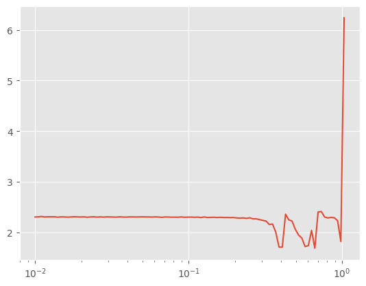

Better! Let’s try training with 0.25.

model = CNN()
model.apply(init_weights)
stats = StoreModuleStatsCB(mods=model.layers)
cbs = [
    MetricsCB(MulticlassAccuracy(num_classes=10)),
    DeviceCB(),
    ProgressCB(plot=True),
    MomentumCB(),
    stats,
]
TrainLearner(
    model,
    fashion_mnist(),
    F.cross_entropy,
    lr=0.25,
    cbs=cbs,
).fit(2)

MulticlassAccuracy	loss	epoch	train
0.549	1.430	0	train
0.673	0.951	0	eval
0.749	0.665	1	train
0.752	0.646	1	eval

stats.mean_std_plot()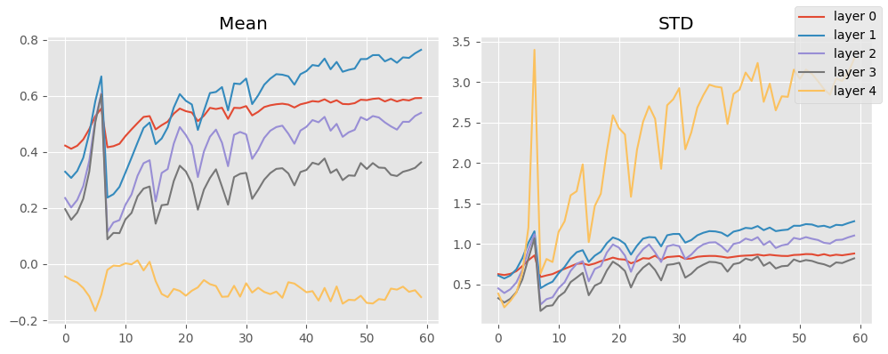

That’s okay! Keep in mind, I did globally normalize the inputs.

Let’s try normalizing batchwise.

---

source

BatchTransformCB

 BatchTransformCB (tfm, on_train=True, on_val=True)

Arbitrarily transform a batch

---

source

NormalizeBatchCB

 NormalizeBatchCB (on_train=True, on_val=True)

Unit normalize a batch

model = CNN()
model.apply(init_weights)
stats = StoreModuleStatsCB(mods=model.layers)
dls = fashion_mnist()
cbs = [
    MetricsCB(MulticlassAccuracy(num_classes=10)),
    DeviceCB(),
    ProgressCB(plot=True),
    NormalizeBatchCB(),
    MomentumCB(),
    stats,
]
learn = TrainLearner(
    model,
    dls,
    F.cross_entropy,
    lr=0.25,
    cbs=cbs,
)
learn.fit(2)

MulticlassAccuracy	loss	epoch	train
0.549	1.398	0	train
0.706	0.823	0	eval
0.758	0.665	1	train
0.769	0.799	1	eval

stats.mean_std_plot()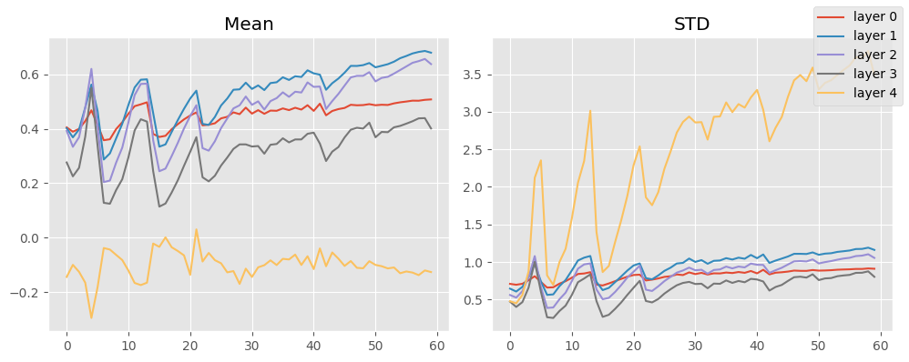

This isn’t much better, unsurprisingly since it was already normalized.

Why aren’t these activation distributions unit normal?

The problem is that StoreModuleStatsCB looks at the output of the ReLU + Convolutional blocks, which cannot output negative numbers (except for the last layer which does not have an non-linearity). Therefore, their output cannot look unit normal!

What if we modified ReLU to allow unit normality?

\[ \text{GeneralReLU}_{l,r,m}(x) = min(\{m, \left. \begin{cases} x & \text{if } x > 0 \\ l \cdot x & \text{otherwise} \end{cases} \right\} - r \}) \]

---

source

GeneralReLU

 GeneralReLU (leak=None, sub=None, max_=None)

Generalized ReLU activation function with normalization and leakiness

This should output a roughly unit normal distribution by pushing all the values down and allowing some contribution from negative values.

x = torch.linspace(-5, 5, steps=100)
gr = GeneralReLU(leak=0.1, sub=0.4)
plt.plot(x, gr(x));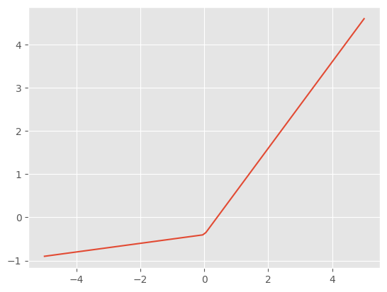

C = Conv2dWithReLU


class CNNWithGeneralReLU(nn.Module):
    """Six layer convolutional neural network with GeneralRelU"""

    def __init__(self, gr=lambda: GeneralReLU(leak=0.1, sub=0.4)):
        super().__init__()
        layers = [  #
            C(1, 8, kernel_size=5, stride=2, padding=2, nonlinearity=gr()),  # 14x14
            C(8, 16, 3, 2, 1, nonlinearity=gr()),  # 7x7
            C(16, 32, 3, 2, 1, nonlinearity=gr()),  # 4x4
            C(32, 64, 3, 2, 1, nonlinearity=gr()),  # 2x2
            nn.Conv2d(64, 10, 3, 2, 1),  # 1x1
        ]
        self.layers = nn.ModuleList(layers)

    def forward(self, x):
        for layer in self.layers:
            x = layer(x)
        *_, w, h = x.shape
        assert w == h == 1
        return rearrange(x, "bs c w h -> bs (c w h)")

⚠️ Now that we are no longer using ReLU outputs, so Kaiming initialization is not acceptable! Luckily, there is an adjustment for this leaky property in the pytorch script

---

source

init_leaky_weights

 init_leaky_weights (module, leak=0.0)

leak = 0.1
model = CNNWithGeneralReLU(gr=lambda: GeneralReLU(leak=leak, sub=0.4))
model.apply(partial(init_leaky_weights, leak=leak))
stats = StoreModuleStatsCB(mods=model.layers)
cbs = [
    MetricsCB(MulticlassAccuracy(num_classes=10)),
    DeviceCB(),
    ProgressCB(plot=True),
    NormalizeBatchCB(),
    MomentumCB(),
    stats,
]
learn = TrainLearner(
    model,
    fashion_mnist(),
    F.cross_entropy,
    lr=0.25,
    cbs=cbs,
)
learn.fit(2)

MulticlassAccuracy	loss	epoch	train
0.656	0.996	0	train
0.762	0.640	0	eval
0.789	0.573	1	train
0.761	0.663	1	eval

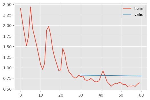
stats.mean_std_plot()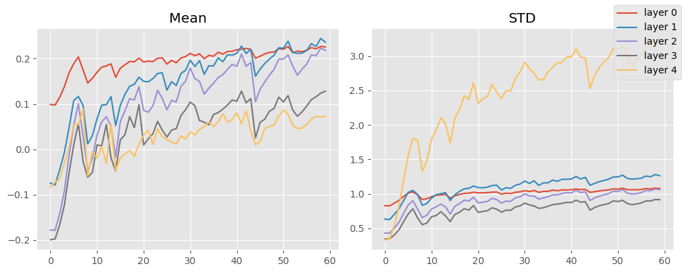

That looks GREAT 🤩 What happens if we keep on training that?

learn.fit(10)

86% accuracy! Not bad.

This goes to show that initialization is underappreciated.

General Initializations

“All You Need Is a Good Init” proposed that there is a generic strategy to initialize any model.

• Setup your model any way you like
• Pass a batch of data through the model and record the layer wise activation statistics
• Apply a unit normalization
• Repeat step 2 until the activation statistics are unit normal within an acceptable tolerance

In code:

---

source

LSUVHook

 LSUVHook (m, tol=0.001)

An abstract hook for performing LSUV for a single layer. .normalize() needs to be implemented for the specific layers

class CNNLSUVHook(LSUVHook):
    def normalize(self):
        if isinstance(self.m, (nn.Conv2d)):
            # Final layer
            self.m.bias -= self.mean
            self.m.weight.data /= self.std
        else:
            self.m.conv.bias -= self.mean
            self.m.conv.weight.data /= self.std

---

source

LSUVInitialization

 LSUVInitialization (mods=None, mod_filter=<function noop>, on_train=True,
                     on_valid=False, hook_cls=<class '__main__.LSUVHook'>)

Layer wise sequential unit variance initialization

leak = 0.1
model = CNNWithGeneralReLU(gr=partial(GeneralReLU, leak=leak))

# Note that we're removing the `model.apply` in favor of LSUVInitialization

stats = StoreModuleStatsCB(mods=model.layers)
cbs = [
    MetricsCB(MulticlassAccuracy(num_classes=10)),
    DeviceCB(),
    ProgressCB(plot=True),
    NormalizeBatchCB(),
    MomentumCB(),
    LSUVInitialization(mods=model.layers, hook_cls=CNNLSUVHook),
    stats,
]
learn = TrainLearner(
    model,
    dls,
    F.cross_entropy,
    lr=0.25,
    cbs=cbs,
)
learn.fit(2)

Layer 0 normalized after 36 batches (0.00, 1.00)
Layer 1 normalized after 37 batches (0.00, 1.00)
Layer 2 normalized after 35 batches (0.00, 1.00)
Layer 3 normalized after 37 batches (0.00, 1.00)
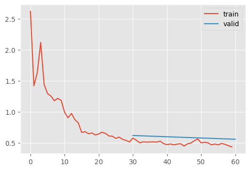
Layer 4 normalized after 2 batches (-0.00, 1.00)

MulticlassAccuracy	loss	epoch	train
0.515	1.553	0	train
0.611	1.258	0	eval
0.710	0.928	1	train
0.749	0.779	1	eval

stats.mean_std_plot()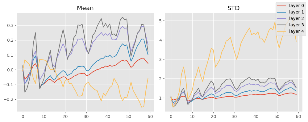

That’s the most accurate yet! The moments look perfect.

Batch and layer normalization

We have been normalizing the inputs before training, but the input distribution can change during training. This is known as internal covariate shift. Can we compensate?

Indeed, we can simply normalize as part of the model architecture

LayerNorm

Proposed one year after BatchNorm by Hinton, but simpler so we’ll start with that. Quite simply implemented like so

class LayerNorm(nn.Module):
    def __init__(self, eps=1e-5):
        super().__init__()
        self.k = nn.Parameter(torch.tensor(1.0))
        self.a = nn.Parameter(torch.tensor(0.0))
        self.eps = eps

    def forward(self, x):
        m = x.mean((1, 2, 3), keepdim=True)
        v = x.var((1, 2, 3), keepdim=True)
        x = (x - m) / ((v + self.eps).sqrt())
        return x

Jeremy notes that:

• Although epsilon is used commonly to correct for the “dead unit” issue, you should not rely on the defaults. Often, they are too small.
• This is not really a “normalization” because k and a can be anything; the network is learning the apropriate distribution moments – and perhaps this is easier for the network

---

source

Conv2dGeneral

 Conv2dGeneral (*args, nonlinearity=<function relu>, norm=None,
                stride:Union[int,Tuple[int,int]]=1,
                padding:Union[str,int,Tuple[int,int]]=0,
                dilation:Union[int,Tuple[int,int]]=1, groups:int=1,
                bias:bool=True, padding_mode:str='zeros', device=None,
                dtype=None)

Convolutional neural network with a built in activation

class CNNWithGeneralReLUAndLayerNorm(nn.Module):
    """Six layer convolutional neural network with GeneralRelU"""

    def __init__(self, gr=GeneralReLU, norm=LayerNorm):
        super().__init__()
        layers = [
            C(1, 8, kernel_size=5, stride=2, padding=2, nonlinearity=gr(), norm=norm()),
            C(8, 16, 3, 2, 1, nonlinearity=gr(), norm=norm()),
            C(16, 32, 3, 2, 1, nonlinearity=gr(), norm=norm()),
            C(32, 64, 3, 2, 1, nonlinearity=gr(), norm=norm()),
            nn.Conv2d(64, 10, 3, 2, 1),  # 1x1
        ]
        self.layers = nn.ModuleList(layers)

    def forward(self, x):
        for layer in self.layers:
            x = layer(x)
        *_, w, h = x.shape
        assert w == h == 1
        return rearrange(x, "bs c w h -> bs (c w h)")

leak = 0.1
model = CNNWithGeneralReLUAndLayerNorm(gr=partial(GeneralReLU, leak=leak))
model.apply(partial(init_leaky_weights, leak=leak))
stats = StoreModuleStatsCB(mods=model.layers)
cbs = [
    MetricsCB(MulticlassAccuracy(num_classes=10)),
    DeviceCB(),
    ProgressCB(plot=True),
    NormalizeBatchCB(),
    MomentumCB(),
    stats,
]
learn = TrainLearner(
    model,
    dls,
    F.cross_entropy,
    lr=0.25,
    cbs=cbs,
)
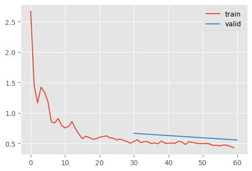
learn.fit(2)

MulticlassAccuracy	loss	epoch	train
0.666	0.985	0	train
0.779	0.621	0	eval
0.819	0.501	1	train
0.801	0.561	1	eval

Even more accurate, by a bit.

While this does help, it turns out that BatchNorm and LayerNorm introduces complixities that have led to me lose favor recently. This just means that the initialization is even more important, as a skill.

That being said, here’s the code for BatchNorm.

---

source

BatchNorm

 BatchNorm (num_filters, mom=0.1, eps=1e-05)

Batch normalization

What does lerp_ do here?

momentum = 0.5
torch.lerp(tensor(1.0), tensor(2.0), tensor(momentum))

tensor(1.5000)

momentum = 0.3333
torch.lerp(tensor(1.0), tensor(2.0), tensor(momentum))

tensor(1.3333)

The basic idea is to normalize the batches accourding to the weighted average of the means and variances of the previous batches. Hopefully, this makes it such that if the model encounters a “weird” batch, it’s not thrown off too much.

---

source

CNNWithGeneralReLUAndBatchNorm

 CNNWithGeneralReLUAndBatchNorm (gr=<class '__main__.GeneralReLU'>)

Six layer convolutional neural network with GeneralRelU

leak = 0.1
model = CNNWithGeneralReLUAndBatchNorm(gr=partial(GeneralReLU, leak=leak))
model.apply(partial(init_leaky_weights, leak=leak))
stats = StoreModuleStatsCB(mods=model.layers)
cbs = [
    MetricsCB(MulticlassAccuracy(num_classes=10)),
    DeviceCB(),
    ProgressCB(plot=True),
    NormalizeBatchCB(),
    MomentumCB(),
    stats,
]
learn = TrainLearner(
    model,
    dls,
    F.cross_entropy,
    lr=0.25,
    cbs=cbs,
)
learn.fit(2)

MulticlassAccuracy	loss	epoch	train
0.702	0.845	0	train
0.769	0.666	0	eval
0.817	0.503	1	train
0.806	0.556	1	eval

Just a tiny bit better, but that looks very smooth. Let’s see if we can increase the learning rate.

model = CNNWithGeneralReLUAndBatchNorm(gr=partial(GeneralReLU, leak=leak))
model.apply(partial(init_leaky_weights, leak=leak))
learn = TrainLearner(
    model,
    dls,
    F.cross_entropy,
    lr=0.4,
    cbs=cbs,
)
learn.fit(2)

MulticlassAccuracy	loss	epoch	train
0.419	1.934	0	train
0.172	193.459	0	eval
0.399	2.227	1	train
0.100	2.383	1	eval

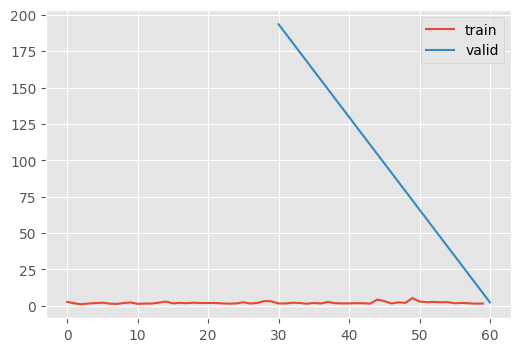
Nope…

Towards 90%

Let’s try a few different things:

• Lower batch size
• Decrease learning rate (smaller batch sizes neccesitate lower learning rates)
• Train for longer
• Finetune with an even lower learning rate

model = CNNWithGeneralReLUAndBatchNorm(gr=partial(GeneralReLU, leak=leak))
model.apply(partial(init_leaky_weights, leak=leak))
learn = TrainLearner(
    model,
    fashion_mnist(256),
    F.cross_entropy,
    lr=0.2,
    cbs=cbs,
)
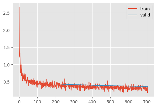
learn.fit(3)

MulticlassAccuracy	loss	epoch	train
0.817	0.504	0	train
0.848	0.426	0	eval
0.870	0.356	1	train
0.862	0.385	1	eval
0.883	0.319	2	train
0.870	0.362	2	eval

learn = TrainLearner(
    model,
    fashion_mnist(256),
    F.cross_entropy,
    lr=0.05,
    cbs=cbs,
)
learn.fit(2)

MulticlassAccuracy	loss	epoch	train
0.900	0.276	0	train
0.882	0.328	0	eval
0.903	0.267	1	train
0.886	0.324	1	eval

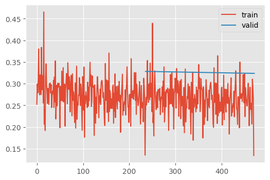
88%! So close. We’ll get there in the next notebook.