import matplotlib

matplotlib.rcParams["image.cmap"] = "gray_r"Denoising Diffusion Implicit Modeling
In this module, we improve the sampling algorithm to further improve the realism and speed of our Generative Fashion MNIST model
Adapted from
Training a model
To start with, let’s train a model like the DDPM V3 notebook and try to achieve our best FID yet.
fashion_unet
def fashion_unet(

):
fp = Path("../models/fashion_unet_2x.pt")
ddpm = DDPM(βmax=0.01)  # 👈 reduce maximum beta
if fp.exists():
    unet = torch.load(fp)
else:
    unet = fashion_unet()
    train(
        unet,
        lr=1e-2,  # 👈 increase the maximum learning rate
        n_epochs=25,  # 👈 dramatically increase the number of epochs
        bs=128,
        opt_func=partial(torch.optim.Adam, eps=1e-5),  # 👈 increase Adam epsilon
        ddpm=ddpm,
    )
    torch.save(unet, fp)
We also want a sampler that’s quite fast, so we’ll re-use the predicted noise
sample
def sample(
    ddpm, model, n:int=16, device:str='cpu', return_all:bool=False
):
x_ts, x_0s = sample(ddpm, unet, return_all=True, n=256)100%|██████████████████████████████████████████████████████████████████████████████████████████████████████████████████████████████████████| 999/999 [00:29<00:00, 34.38time step/s]CPU times: user 11.6 s, sys: 13 s, total: 24.6 s
Wall time: 29.2 sanimate
def animate(
    imgs
):
animate([*x_0s[::25], x_0s[-1]])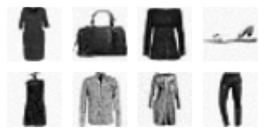
ImageEval.fashion_mnist?Signature: ImageEval.fashion_mnist(fp='../models/fashion_mnist_classifier.pt', bs=512) Docstring: <no docstring> File: ~/Desktop/SlowAI/nbs/slowai/fid.py Type: method
img_eval = ImageEval.fashion_mnist(bs=256)
img_eval.fid(x_0s[-1])936.2686767578125Diffusers API
Now, for comparison, we’ll use the diffusers API.
diffusers_sample
def diffusers_sample(
    sched, sz:tuple=(256, 1, 32, 32), skip_steps:NoneType=None, kwargs:VAR_KEYWORD
):
sched = DDPMScheduler(beta_end=0.01)
sched.set_timesteps((1000 - 50) // 3 + 50)
x_t = diffusers_sample(sched)
100%|█████████████████████████████████████████████████████████████████████████████████████████████████████████████████████████████████████████████| 366/366 [00:21<00:00, 17.04it/s]CPU times: user 22.4 s, sys: 60.8 ms, total: 22.5 s
Wall time: 21.5 sshow_images(x_t[:8, ...], imsize=0.8)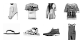
img_eval.fid(x_t)1133.3358154296875For DDIM:
sched = DDIMScheduler(beta_end=0.01)
sched.set_timesteps((1000 - 50) // 3 + 50)
x_t = diffusers_sample(sched)
100%|█████████████████████████████████████████████████████████████████████████████████████████████████████████████████████████████████████████████| 366/366 [00:21<00:00, 16.98it/s]CPU times: user 22.5 s, sys: 69.2 ms, total: 22.6 s
Wall time: 21.6 sshow_images(x_t[:8, ...], imsize=0.8)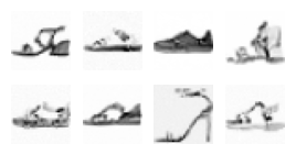
img_eval.fid(x_t)1313.16455078125It turns out, these are similar quality.
DDIM, algorithm
The basic idea is that different time steps may benefit from having different amounts of noise.
This article does a good job of explaining the motivation.
In either algorithm, we determine the predicted noise, scale the predict apropriately for the time step, remove it from the latent representation and scale the sum.
\[ \hat{x}_0 = \frac{x_t - \sqrt{1-\bar{\alpha}_t} \epsilon_{\theta}(x_t)}{ \sqrt{ \bar{\alpha}_t } } \]
Then, for DDPM, we re-add a fixed amount of noise to predict \(x_{t-1}\). For DDIM, we add noise as a function of \(\sigma\). (Because this can be made stochastic or deterministic, but the training objective is compatible, the name was changed to Denoising Diffusion Implicit Model.)
\[ q_\sigma ( x_{t-1} | x_t, x_0 ) = \mathcal{N} \left( \sqrt{\bar{\alpha}_{t-1}} x_0 + \sqrt{ 1 - \bar{\alpha}_{t-1} - \sigma_t^2 } \cdot \frac{x_t - \sqrt{\bar{\alpha}_t} x_0}{\sqrt{1-\bar{\alpha_t}}}, \sigma_t^2 I \right) \]
We can rewrite this in terms of \(x_{t-1}\), which is what we need to calculate for each step. This is composed of:
- Predicted \(x_0 = \left( \frac{x_t - \sqrt{1-\bar{\alpha}_t} \epsilon_{\theta}^{(t)} }{\sqrt{ \bar{\alpha}_t }} \right)\) (this is the same as DDPM)
- Direction towards \(x_t = \sqrt{ 1 - \bar{\alpha}_{t-1} - \sigma^{2}_{t} } \cdot \epsilon_{\theta}^{(t)} (x_t)\)
- Random noise \(= \sigma_t \epsilon_t\)
\[ x_{t-1} = \sqrt{ \bar{\alpha}_{t-1} } \left( \frac{x_t - \sqrt{1-\bar{\alpha}_t} \epsilon_{\theta}^{(t)} }{\sqrt{ \bar{\alpha}_t }} \right) + \sqrt{ 1 - \bar{\alpha}_{t-1} - \sigma^{2}_{t} } \cdot \epsilon_{\theta}^{(t)} (x_t) + \sigma_t \epsilon_t \]
and
\[ \begin{align*} \sigma_t &= \eta \sqrt{(1-\bar{\alpha}_{t-1}) / (1-\bar{\alpha}_t)} \sqrt{1-\bar{\alpha_t} / \bar{\alpha}_{t-1}} \\ \eta &\in [0,1] \end{align*} \]
Typically, we use an \(\eta\) parameter to interpolate between DDPM and DDPM, where \(\eta=1\) corresponds to DDIM; if \(\sigma_t=0\), this corresponds to DDPM.
DiffusersStyleDDIM
def DiffusersStyleDDIM(
    n_steps:int=1000, βmin:float=0.0001, βmax:float=0.02, η:float=1.0, # η is eta
):
Modify the training behavior
DiffusersStyleDDPM
def DiffusersStyleDDPM(
    n_steps:int=1000, βmin:float=0.0001, βmax:float=0.02
):
Modify the training behavior
DDIMOutput
def DDIMOutput(
    prev_sample:Tensor
)->None:
This is nice because the only parameters are \(\bar{\alpha}\) and \(\eta\).
sched = DiffusersStyleDDIM(βmax=0.01)
skip_steps = list(sched.timesteps)[:-50]
skip_steps = skip_steps[1::3] + skip_steps[2::3]
len(skip_steps)632x_t = diffusers_sample(sched, skip_steps=skip_steps)100%|█████████████████████████████████████████████████████████████████████████████████████████████████████████████████████████████████████████████| 999/999 [00:22<00:00, 44.14it/s]CPU times: user 23.5 s, sys: 123 ms, total: 23.6 s
Wall time: 22.6 sshow_images(x_t[:8, ...], imsize=0.8)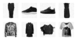
img_eval.fid(x_t)913.7852783203125sched = DiffusersStyleDDIM(βmax=0.01)
steps = list(sched.timesteps)
skip_steps = {step for step in steps if step not in steps[::10] and step > 50}
x_t = diffusers_sample(sched, skip_steps=skip_steps)100%|████████████████████████████████████████████████████████████████████████████████████████████████████████████████████████████████████████████| 999/999 [00:09<00:00, 102.68it/s]CPU times: user 10.7 s, sys: 72.3 ms, total: 10.7 s
Wall time: 9.73 sshow_images(x_t[:8, ...], imsize=0.8)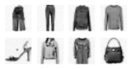
img_eval.fid(x_t)900.450927734375This gives us a slight improvement in FID and a 2x increase in speed.